Welcome to MET_waves’s documentation!
Tools for data analysis and visualization of MET Norway (https://www.met.no/) wave datasets (e.g., NORA3, WAM4).
Installing MET_waves
Install anaconda3 or miniconda3
Clone MET_waves:
$ git clone https://github.com/KonstantinChri/MET_waves.git
$ cd MET_waves/
Create the environment with the required dependencies and install MET_waves:
$ conda config --add channels conda-forge
$ conda env create -f environment.yml
$ conda activate MET_waves
$ pip install -e .
Examples
The package is under preparation. Some examples are given below:
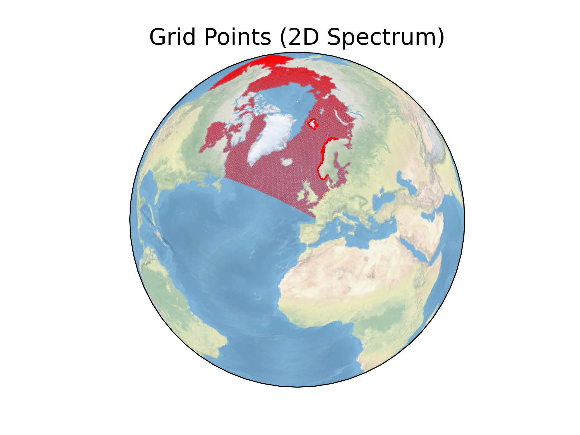
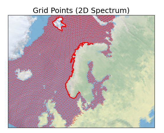
Plot all grid points that spectrum is available in NORA3/WAM4/WW3 datasets (https://thredds.met.no):
# example for NORA3:
from MET_waves import plot_grid_spec_points
url = 'https://thredds.met.no/thredds/dodsC/windsurfer/mywavewam3km_spectra/2020/12/SPC2020123100.nc'
plot_grid_spec_points(url,s=0.01,color='red')
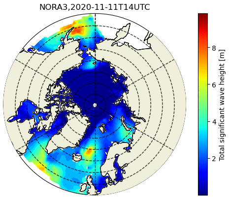
Plot panarctic map using NORA3 data (use method=’mean’ to average over time or method=’timestep’ to get each timestep):
from MET_waves import plot_panarctic_map
plot_panarctic_map(start_time='2020-11-11T14', end_time='2020-11-11T15',
                   product='NORA3', variable='hs', method='timestep')
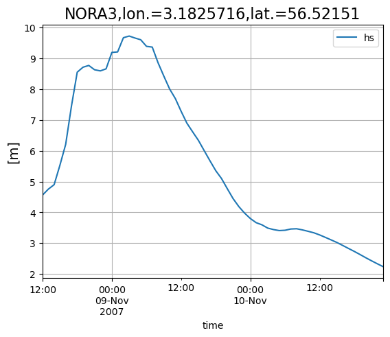
Plot time series of a NORA3 grid point (and write data to .csv if write_csv=True):
from MET_waves import plot_timeseries
plot_timeseries(start_time='2007-11-08T12', end_time='2007-11-10T23',
                lon=3.20, lat=56.53, product='NORA3',
                variable='hs', write_csv=True, ts_obs=None)
Since the program uses directly thredds.met.no to access the data, it can take some time to plot/extract very long time series. For long time series, please use the following function that extracts times series of the nearest gird point (lon,lat) from a wave product and saves it in a netcdf format:
from MET_waves import extract_ts_point
extract_ts_point(start_date ='2019-01-01',
                 end_date= '2019-01-31',
                 variable=['hs','tp','hs_swell','tp_swell', 'ff'],
                 lon = 5, lat = 60,
                 product='NORA3')
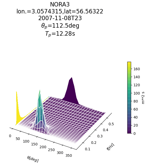
Plot 2D spectra of a NORA3(product=’SPEC_NORA3’)/WW3(product=’SPEC_WW3’) grid point:
from MET_waves import plot_2D_spectra
plot_2D_spectra(start_time='2007-11-08T23', end_time='2007-11-10T23',
                lon=3.20, lat=56.53, product='SPEC_NORA3')
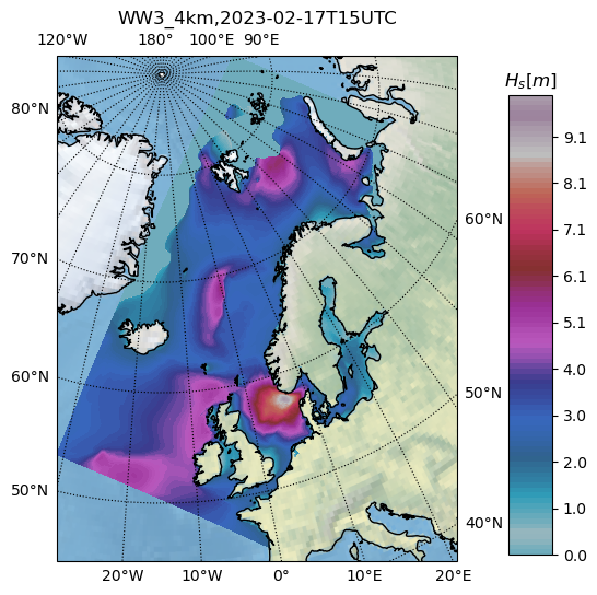
Plot WW3_4km forecast:
from MET_waves import plot_MET_forecast
plot_MET_forecast('https://thredds.met.no/thredds/dodsC/ww3_4km_archive_files/2023/02/17/ww3_4km_20230217T06Z.nc')
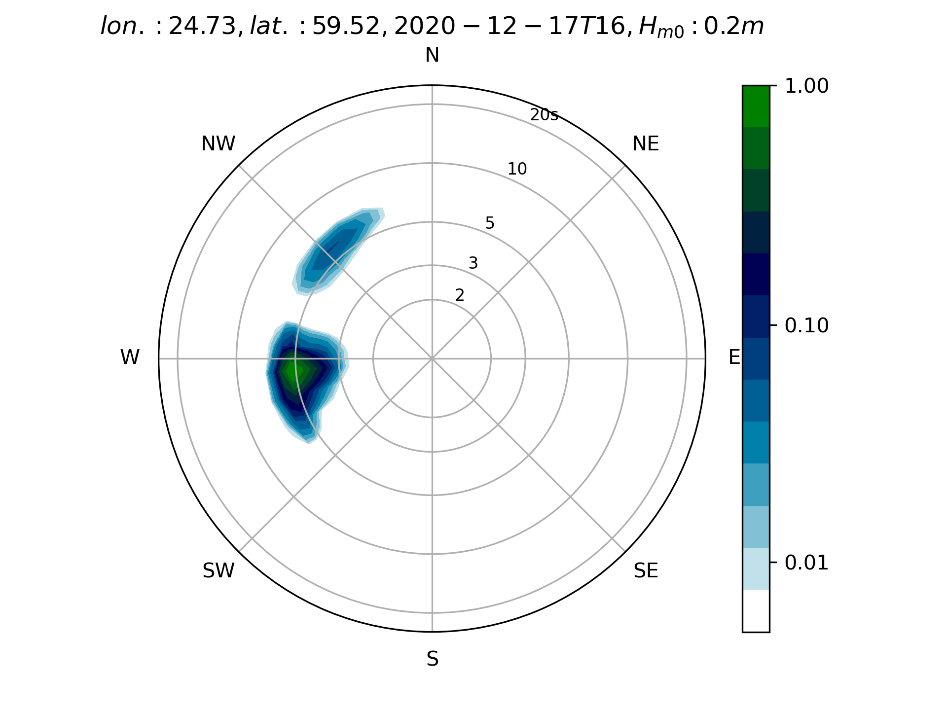
Plot SWAN 2D spectrum:
from MET_waves import plot_swan_spec2D
plot_swan_spec2D(start_time='2020-12-17T16', end_time='2020-12-17T17',infile='SWAN_spec.nc', site=0)
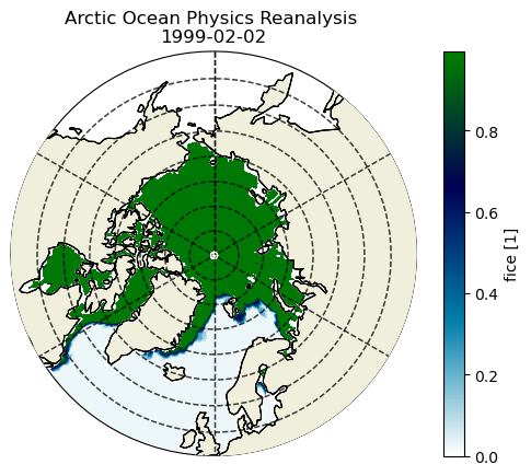
Plot TOPAZ data (use method=’mean’ to average over time or method=’timestep’ to get each timestep):
from MET_waves import plot_topaz
plot_topaz(start_time='1999-02-02',end_time='1999-02-03',
           variable='fice',method = 'timestep',save_data =True)